Event Study Application Blueprint
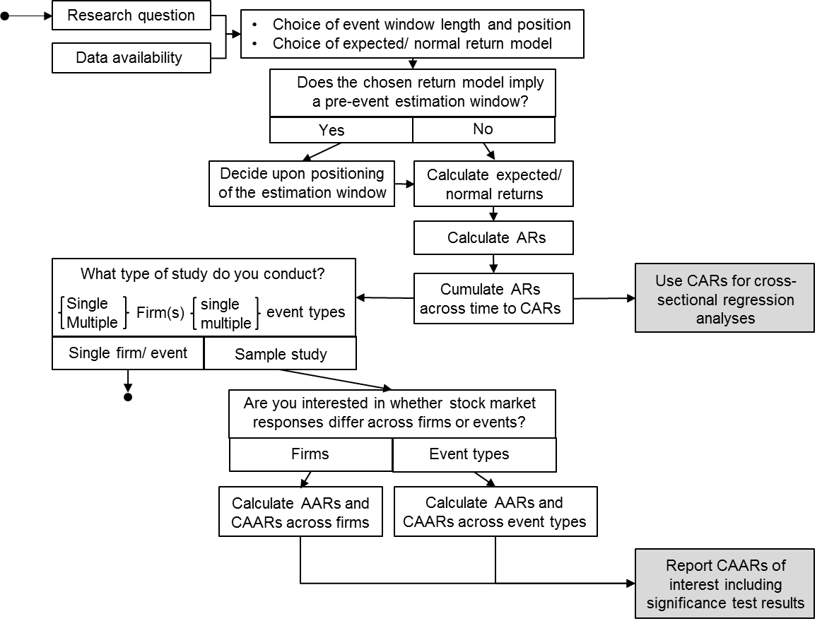
Event studies follow a uniform workflow ("blueprint") that consists of methodological choices and analytical steps. While researchers may use some type of dedicated tool for the analysis, they should be knowledgeable about the overall workflow and its implied choices. Figure 1 illustrates this event study blueprint. It is preceded by a description of its inherent methodological choices and analytical steps.
- Choose an expected/normal return model that matches your research question and data availability
- To set the event window length and the position of the event window, answer the following questions: On what date did the market receive the information about the event you want to study? Has there been potential information leakage prior and a certain market pricing/digestion period subsequent to the date?
- Calculate expected/normal returns (i.e., returns for the firms' stocks assuming the event had not taken place)
- Calculate abnormal returns (ARs) as the difference between the observed returns and the 'normal/ no-news' returns for each firm and day in the event window
- These single-day 'abnormal returns' can then be further aggregated across time to 'cumulative abnormal returns' (CARs) or cross-sectionally to 'average abnormal returns' (AARs). Aggregating the abnormal returns across both time and firms yields the 'cumulative average abnormal returns' (CAARs).
- In a final step, calculate significance tests to establish whether the abnormal returns found at any of the AR-, AAR-, CAR- or CAAR-levels are statistically valid/significant
Figure 1: Event Study Blueprint
Own Illustration
Choosing the Lengths of the Estimation and Event Windows
Depending on the choice of expected/normal return model, event studies either imply the use of an event window only (e.g., the market-adjusted model) or an event and an estimation window (e.g., the market model). Most common, the 'market model' is used. It predicts normal returns with a regression analysis that regresses stock returns on market returns over the 'estimation window'. Through this analysis, the typical relationship between the stock and its reference index is captured in two parameters (i.e., alpha, beta). Figure 2 sketches the data structure used by event studies and provides further information on how this data structure is used by the 'market model'.
Figure 2: Data Structure of Event Studies with an Estimation Window

Adapted from Benninga (2008: 372)
Allocating the estimation and event windows poses two major challenges to scholars. First, they must identify the correct event date as an 'anchor' for the whole analysis, and second, they need to specify the lengths and positions of the estimation and event windows.
Identifying the event date is not always a simple task. In the analysis of M&A transactions, for example, initial rumors about the transaction are typically followed by an official announcement and a closing of the transaction. On each of these events, information is released, posing the question which date represents the correct event date to be analyzed. Scholars investigating this issue found the information content of the first official announcement being highest and therefore representing the correct event date in the context of M&A studies (Dodd, 1980). Similar questions also arise when studying other event types.
Further, there is no definite rule on the length of an event study's estimation and event windows. Researchers have a discretionary choice when deciding about these parameters. The challenge researchers have to solve, with regard to the estimation window, is to find the balance in the tradeoff between improved estimation accuracy and potential parameter shifts. Longer estimation windows promise greater accuracy, as they imply larger samples of returns, but they also bear the risk of covering structural breaks (e.g., due to confounding events) of the $\alpha$ and $\beta$ factors, which will lead to biased estimators. A similar challenge exists with the event window, as one needs to specify over which period the studied event impacted the respective stock. On the one hand, information leakage and longer information processing periods favor longer event windows, and on the other hand, confounding events suggest shorter event windows.
Recent meta-research reviewing 400 event studies finds that estimation window lengths spread out between 30 and 750 days (Holler, 2014). Studies investigating the sensitivity of results (e.g., the predicted return on the event date) suggest that results are not sensitive to varying estimation window lengths as long as the window lengths exceed 100 days (Armitage, 1995, Park, 2004). Event windows typically range in their length between 1 and 11 days and center symmetrically around the event day (Holler, 2014). The most common choice of event window length in a recent paper by Oler, Harrison, and Allen (2007) is 5 days, representing 76.3% of the reviewed studies.
References and additional links
Benninga, S. 2008. Financial modeling (3 ed.). Boston, MA: MIT Press.